Connection network buying guide: copper, fiber, transceivers

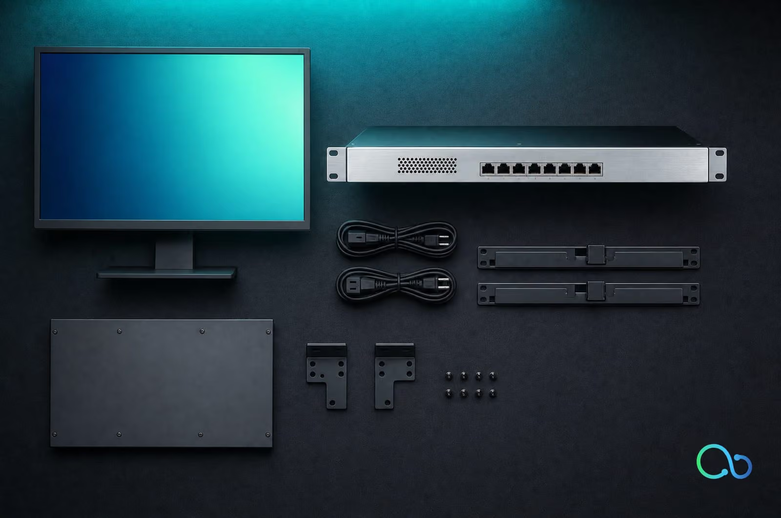
Understanding the connection network layer in data‑center environments

Servers, storage arrays, and switches must exchange traffic at predictable rates. The connection network provides the physical pathways that carry Ethernet frames, Fibre Channel packets, or management traffic between these devices. It sits at the physical layer (OSI Layer 1) and defines cable type, connector geometry, and signaling standards that determine reach, bandwidth, and error tolerance.

A connection network is not a logical topology; it is the collection of cables, transceivers, and patch panels that enforce the electrical or optical specifications required by the attached equipment. Copper solutions such as Cat6a or Cat8 use twisted‑pair conductors and RJ‑45 connectors, supporting 10 GbE up to 100 m or 25 GbE over shorter runs. Fiber options include OM3/OM4 multimode for 10 GbE–40 GbE within a rack, and OS2 single‑mode for 100 GbE across longer distances. Each medium imposes a maximum bend radius, insertion loss budget, and temperature range that must be respected during rack layout.

Connector form factors also affect density. QSFP28 modules occupy 4 × 4 mm footprints on a switch front panel, while SFP+ modules use 2 × 2 mm footprints, allowing higher port counts per chassis. When planning a connection network, verify that the chosen cabling and transceiver families match the switch and server port specifications, and that the physical infrastructure (cable trays, conduit, and patch panels) can accommodate the required bend radii and strain relief. Detailed product families are listed in the network cables catalog.

Copper cabling options and their impact on cost and density

Category‑5e (Cat‑5e)

Cat‑5e supports 100 MHz signaling and a maximum of 1 GbE over 100 m (328 ft). The cable is unshielded twisted pair (UTP) in a 24‑AWG construction, which keeps material cost low. Typical 1 GbE server NICs and entry‑level top‑of‑rack switches provide 24 × 1 GbE ports per chassis. Because the cable can only carry 1 GbE reliably, higher‑density 10 GbE deployments usually require a different standard.

Category‑6 (Cat‑6)

Cat‑6 raises the signaling frequency to 250 MHz and can sustain 10 GbE for up to 55 m (180 ft) on standard UTP, or 100 m when using shielded twisted pair (STP) with stricter installation practices. The tighter twist and optional foil shielding increase material cost modestly compared with Cat‑5e. Many mid‑range switches ship with 48 × 1 GbE or 24 × 10 GbE ports, allowing a higher port density while still using copper. When planning a rack, verify that the run length from the switch to each server stays within the 55 m limit for reliable 10 GbE.

Category‑6a (Cat‑6a)

Cat‑6a extends the bandwidth to 500 MHz and guarantees 10 GbE over the full 100 m (328 ft) distance. The cable uses a larger 23‑AWG conductor and typically includes overall shielding (S/FTP) to control crosstalk. Material cost is higher, and the thicker jacket can affect cable management density in dense rack environments. High‑performance switches often expose 48 × 10 GbE ports, and modern NICs frequently ship with dual‑port 10 GbE or 25 GbE options that still rely on Cat‑6a for short‑haul connections.

When comparing the three standards, consider the required link speed, maximum run length, and the physical space available for cable bundles. For most data‑center deployments that need 10 GbE across a full rack, Cat‑6a provides the most predictable performance, while Cat‑5e remains the lowest‑cost choice for 1 GbE back‑plane links. Detailed switch port configurations can be reviewed in the network‑switches catalog.

Fiber cabling and optical transceiver families

Single‑mode fiber (SMF) uses a 9 µm core and propagates light in a single ray. It supports distances from 2 km to 80 km at 1310 nm or 1550 nm, making it the choice for inter‑data‑center links or campus backbones. Multimode fiber (MMF) has a larger 50 µm or 62.5 µm core, allowing multiple propagation modes. Typical MMF standards—OM3 (850 nm, up to 300 m) and OM4 (850 nm, up to 400 m)—are suited for intra‑rack or intra‑aisle connections where cost and ease of termination are priorities.

Optical transceivers translate electrical signals to light and back. The most common form factors are:

Form factor	Lane count	Typical data rate per lane	Max power draw*
SFP	1	1 GbE, 10 GbE	≤ 1 W
SFP+	1	10 GbE	≤ 1.5 W
QSFP	4	40 GbE (4 × 10 GbE)	≤ 4 W
QSFP28	4	100 GbE (4 × 25 GbE)	≤ 5 W

*Power consumption varies with manufacturer and signaling speed.

SFP modules fit a 19 mm × 13.5 mm footprint and are ideal for low‑density ports. SFP+ retains the same size while adding 10 GbE capability, allowing a simple upgrade without changing the chassis. QSFP expands the footprint to 42 mm × 18 mm, providing four lanes in a single slot; this reduces port density but simplifies cabling for 40 GbE or 100 GbE aggregates. QSFP28 uses the same chassis as QSFP but supports higher lane rates, demanding tighter thermal design.

When selecting a transceiver, match the fiber type to the module’s wavelength (e.g., 1310 nm for SMF, 850 nm for MMF) and verify that the switch or server can supply the required power budget. For a concise comparison of SFP, SFP+, and QSFP options, see the simple guide for enterprise fiber networking.

Designing redundancy and topology for resilience

Leaf‑spine

A leaf‑spine fabric isolates east‑west traffic to two hops. Each leaf switch connects to every spine node with multiple uplinks. To meet a N+1 redundancy target, provision at least two 40 GbE or 100 GbE links per leaf‑spine pair. Use QSFP‑28 or OSFP transceivers for the uplinks and match the cable type to the distance: direct‑attach copper (DAC) for runs under 7 m, MPO‑MTP multimode fiber for 30‑m spans, and single‑mode fiber with LC or MPO connectors for longer paths. Selecting identical transceiver modules on both ends simplifies inventory and spare‑part management.

Ring

A ring topology provides a single failure path by looping traffic back around the loop. When implementing a dual‑ring, each node requires two independent links to its neighbors. For 10 GbE rings, SFP+ transceivers paired with OM3 multimode fiber (850 nm) support up to 300 m, while for 25 GbE or 40 GbE rings, use SFP28 or QSFP‑28 modules with appropriate single‑mode fiber (1310 nm) to stay within loss budgets. Ensure the chosen transceiver family supports bidirectional operation if the switch vendor offers that mode, reducing the number of fibers needed.

Dual‑homed

Dual‑homed servers or storage arrays connect to two separate aggregation switches. This approach isolates a single switch failure without affecting the host. Match the host NIC speed to the uplink: a 25 GbE NIC should use an SFP28 transceiver and compatible fiber or DAC, while a 100 GbE NIC uses a QSFP‑28 module. When both links terminate on different switch vendors, verify that the transceiver form factor and wavelength are supported on each platform.

Across all topologies, maintain a spare pool of transceivers that match the installed form factor and wavelength. Keeping a balanced stock of DACs, MPO‑MTP cables, and single‑mode LC modules reduces downtime when a link fails. For detailed compatibility tables, refer to the network adapters catalog.

Procurement considerations and spare‑part strategies

Evaluating total cost of ownership

When comparing copper and fiber options, include more than the per‑port price. Account for power consumption of active optics, cooling load in the rack, and the expected replacement cycle of transceivers. A 10 GbE SFP+ module typically consumes 0.5 W, while a 40 GbE QSFP+ can draw up to 3 W per port; the higher draw translates into additional PDU capacity and airflow requirements. Factor in the cost of compatible cables—direct‑attach copper (DAC) is inexpensive for short runs but limited to 7 m, whereas MPO‑LC fiber assemblies have higher upfront cost but support longer distances and higher bandwidth without signal loss. Include warranty and support terms from the manufacturer, as a longer warranty reduces the risk of unexpected replacement expense.

Matching port density to growth

Select switches that provide a balance of current utilization and headroom. A 48‑port 1 GbE chassis with optional 10 GbE uplink modules can accommodate a gradual migration to higher speeds without replacing the entire chassis. For new builds, consider modular switches that allow line‑card swaps; a 2 U chassis with 24 × QSFP28 ports can be populated with 100 GbE optics now and later re‑populated with 200 GbE modules as the network scales. Verify that the chosen form factor (SFP, SFP+, QSFP, QSFP28) aligns with the transceiver inventory you plan to keep.

Spare‑part inventory

Maintain a minimum stock of the most common transceiver types and cable assemblies used in the deployment. For a 48‑port edge switch, keep at least two spare SFP+ modules and a matching length of LC‑LC fiber patch cord. Store DACs in anti‑static bags and label each with the supported speed and distance. Rotate inventory every 12 months to avoid aging of optical components.

Next step: Create a spreadsheet that lists each active port type, its power draw, required cable length, and a minimum spare quantity; use this to generate a purchase order for the initial spare‑part stock.

Frequently asked questions

What factors determine copper versus fiber for a connection network?

Copper offers lower upfront cost and easier termination but is limited in distance and bandwidth. Fiber supports longer runs and higher speeds, with higher material cost and stricter handling requirements.

How do I choose between SFP, SFP+, and QSFP transceivers?

Select SFP for 1 GbE, SFP+ for 10 GbE, and QSFP for 40 GbE or 100 GbE links. Match the transceiver form factor to the switch or NIC port and verify the supported wavelength and cable type.

What should I consider for spare‑part inventory?

Stock transceivers that match the most common link speeds in your environment, keep a few of each form factor, and track firmware compatibility to avoid mismatches during replacements.

How does port density affect power and cooling planning?

Higher‑density modules like QSFP consume more power per slot and generate more heat. Ensure the switch chassis can deliver sufficient power per port and that airflow is adequate for the expected load.